Can CPUs leverage sparsity?

In my previous blog post, I discussed our recent announcement that we had leveraged extreme sparsity to improve deep neural network inference performance by over 112X. This performance improvement was achieved on an FPGA platform, where the inherent flexibility of the FPGA allowed the computational efficiencies introduced by sparsity to be fully exploited.

While this is clearly an impressive speedup, it becomes even more impactful when the absolute performance of our sparse models on the FPGA is compared with what is achievable using sparse models on other general-purpose compute platforms.

What is Network Sparsity?

Most current deep learning networks are referred to as ‘dense’ networks. In these dense networks, neurons are highly interconnected and highly active. This combination of both high activity and interconnectedness ensures that numerous computations are required to compute the output of each and every neuron, making the use of these dense networks a costly undertaking requiring significant computational power and incurring unsustainable energy costs.

At Numenta, where we apply insights from neuroscience to improve both the performance and intelligence of machine intelligence systems, we have long recognized that these dense networks bear little resemblance to the human neocortex. In the human neocortex, neuron interconnections are incredibly sparse, with each neuron only connecting to a small fraction of the cortex’s total neurons. Similarly, at any given point, only a couple of percent of neurons are active. We can apply these neuroscience insights to deep learning and create ‘sparse’ neural networks. Incredibly, it is possible to create sparse networks with identical accuracy to a comparable dense network, but in which neurons are connected to as few as 5% of neurons in the previous layer and neuron activations are limited to less than 10%!

As can be readily imagined, the ability to create sparse networks with around 20X fewer connections than the standard dense equivalent, while achieving comparable accuracy, requires sophisticated techniques. This is an active area of research in the AI community, with a wide variety of techniques being proposed and refined in recent years. In many cases, sparse networks are created by first training a dense network and then, as a final step, removing (or ‘pruning’) the least-important neuron connections until the desired level of sparsity is achieved. Typically, some degree of additional fine tuning of the sparse network is required in order to recover the accuracy following the pruning. In contrast, Numenta has focused on techniques that enable the training of sparse networks and has also developed techniques to effectively limit neural activations, enabling the creation of extremely sparse deep neural networks.

In comparison to a corresponding dense network, these extremely sparse networks reduce the number of computations required to compute the output of the network by an order of magnitude or more. As a result, one would expect significant performance and power advantages to be associated with their use. This is exactly what Numenta demonstrated on an FPGA. In this blog, I investigate whether the same holds true for sparse networks on CPUs.

CPUs and ONNX engines

In this blog post, I compare our FPGA sparse model performance with the performance of sparse models running on modern CPUs (I will tackle GPUs in a subsequent blog). To create the sparse models for use on the CPU, I used an open-source library from Microsoft to prune a pre-trained dense network. The resulting CPU sparse network has identical sparsity levels to our sparse networks detailed in the Numenta Whitepaper.

To this end, I used PyTorch to train the baseline dense convolutional neural network (CNN) described in the Whitepaper. This model is a deep CNN model trained on the Google Speech Commands (GSC) data set, which consists of 65,000 one-second-long utterances of keywords spoken by thousands of individuals. The task is to recognize the word being spoken from the audio signal. The model has around 2.5M parameters and achieves 96%+ accuracy.

This PyTorch GSC model was then exported using the open ONNX model interchange format, and peak inference performance was investigated on a 24 core (48 hardware thread) Intel Xeon 8275CL (on AWS, this system is a C5.12xlarge). This processor was chosen because it supports Intel’s latest DL Boost Vector Neural Network Instructions and provides ample memory bandwidth to ensure that compute performance is not unnecessarily constrained by memory bottlenecks. Once the CNN network has been exported to the ONNX format, there are a wide variety of both open-source and commercial CPU inference engines that can be used to run the network. Performance was investigated using several common ONNX inference engines and ML compilers, including:

• Intel OpenVINO
• Microsoft ONNX Runtime
• Apache TVM
• Neural Magic Deep Sparse

These inference engines analyze the network, perform a variety of sophisticated optimizations and produce a customized implementation that is tailored to run the specific network on the target hardware platform. As a result, inference performance using these ONNX engines is significantly faster than is typically achievable in PyTorch (even when using PyTorch TorchScript).

Dense Network Performance

As an initial step, the selected CPU inference engines were used to run the baseline dense GSC model and the inference performance was measured. Results from these experiments are shown in Figure 1. Inference performance is highly dependent on the batch size (basically how many samples are available for the system to process in parallel). Figure 1(a) shows performance obtained for batches that contained just a single sample and Figure 1(b) illustrates performance when a batch of 64 samples is available.

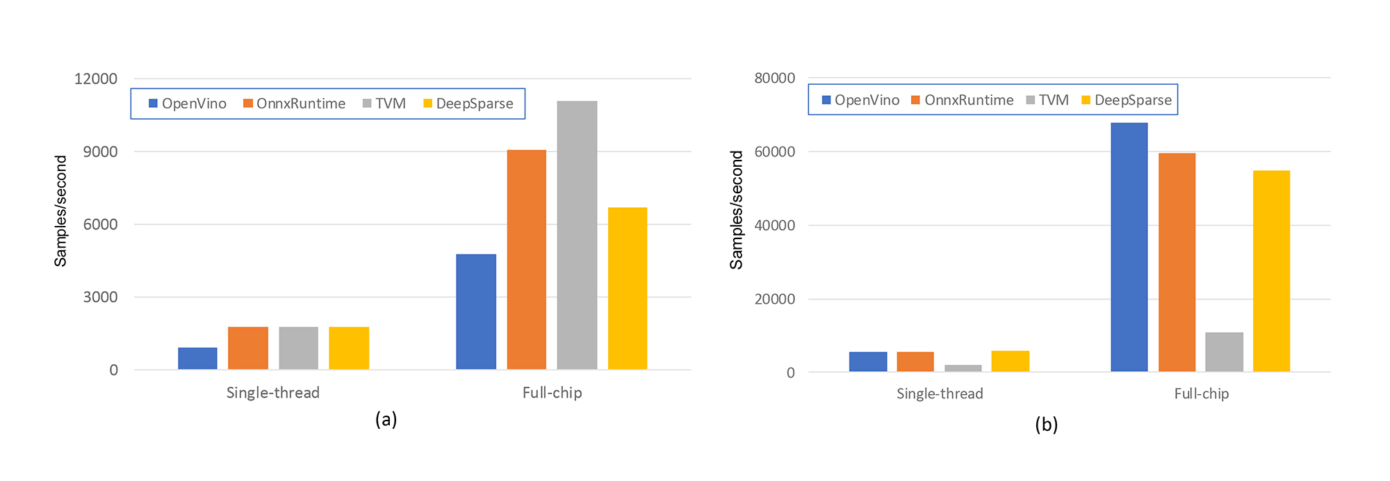
Within Figure 1(a) and Figure 1(b) there are two separate sets of results. The left-most ‘single-thread’ results illustrate the inference performance when the inference engines are constrained to use just one of the 48 hardware threads available. The right-most results illustrate the performance when the engines are allowed to make full use of the entire processor (although they typically needed manual guidance to achieve optimal performance).

There are several interesting observations stemming from the results in Figure 1:

• Even when the batch size is limited to a single sample, allowing the engines to use multiple hardware threads improves performance, illustrating the engines can multithread a single inference operation.
• When multiple samples are available for processing in parallel, the engines can make significantly more efficient use of the available compute resources, even when constrained to using a single hardware thread, as highlighted in Figure 2. Although not shown graphically for space constraints, it was found that, for most inference engines, there are ‘magic numbers’ associated with batch size. Selecting a ‘good’ batch size can increase performance by 20% or more. The chosen batch size of 64 was a magic number.
• TVM appears to produce similar results for both batch sizes, and while it is a performance leader for single-sample inference, it is a clear laggard for the 64 sample runs (if anyone from the Apache TVM project has guidance on whether there are cool flags/options/switches to improve performance that I have omitted, please ping me!).

Impact of model quantization

This initial ONNX model uses 32-bit floating point representations for both model weights and activations. The baseline dense network used on the FPGA used 8-bit integer weights and activations. To enable a fair comparison between the CPU and FPGA performance, I quantized both the weight and activations in the CPU GSC model to eight-bit integers using the tools bundled with the ONNX engines. Remember, this Intel 8275CL processor supports the AVX512 VNNI (Vector Neural Network Instructions) instructions, enabling efficient processing of INT8 quantized networks.

The results obtained for this quantized network are shown in Figure 3 and include a direct comparison with the FPGA performance for the dense network (The FPGA used in these experiments was a Xilinx Alveo™ U250). For clarity, going forward I only show CPU results for a batch size of 64, which in all cases was superior to the single sample results.

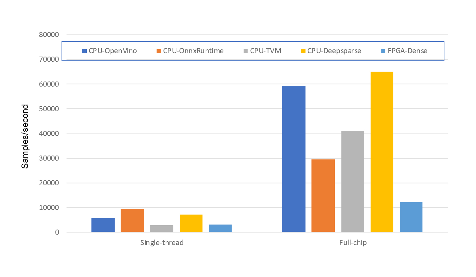
From Figure 3, there are a couple of key observations. Firstly, for the standard dense network, the 24-core CPU outperforms the FPGA by a significant margin. CPUs are optimized for dense, regular computations, and clearly excel! Secondly, comparing the results in Figure 3 with the results in Figure 1, it is clear that, except for the TVM results, the performance improvement from quantization is muted. This is counter to expectations, where a performance improvement of up to 4X could be expected (we are moving from 32-bit floating point operations to 8-bit integer operations, enabling a processor’s 512-bit AVX vector instructions to process 4X more elements in parallel). After investigation, it became apparent that the presence of the maxpool layers in the GSC network is causing problems for the ONNX quantization toolsets. In several instances, manually disabling quantization of certain layers was required to even achieve a speedup! Overall, quantization support in ONNX appears to be still evolving, with many reports of slowdowns, fragility, and non-portability being reported on various ONNX forums.

Sparse model performance

Finally, we can compare the performance of a sparse network running on the CPU with Numenta’s sparse models running on the FPGA. As mentioned previously, in this blog I do not use Numenta’s techniques to create these CPU networks. Our sparse model was optimized for FPGA and won’t run faster on a CPU using existing CPU tools. We are in the process of migrating our approach to CPUs. In this blog, I use the currently available 3rd party tools for creating optimized sparse models for CPU, i.e. based on pruning. Accordingly, to create a sparse version of the model for the CPU, I used Microsoft Neural Network Intelligence software to prune the original dense model. The overall sparsity of the CPU sparse model is 95%, in line with the sparsity used in our FPGA sparse models. In Figure 4, the performance of this sparse model running on the CPU is compared with the Numenta sparse models running on the FPGA.

There are two sparse FPGA results shown in Figure 4, referenced as Numenta-SD and Numenta-SS. These refer to the FPGA sparse networks created by Numenta. Numenta-SD is our sparse-dense model, where the weights are sparse, but activations are considered dense, while Numenta-SS is our sparse-sparse model that fully exploits sparsity in both the weights and activations. The sparse ONNX model used on the CPU is sparse-dense. The ability to simultaneously exploit both weight and activation sparsity on CPUs in a performant manner remains an open problem: The location of the zero weights is known in advance, allowing carefully crafted kernels that exploit their presence to be constructed. The locations of the zero-valued ‘activations’ are dynamic, forcing their position to be computed dynamically at run-time. To my knowledge, no CPU inference engine currently attempts to exploit the multiplicative power of combining the two forms of sparsity.

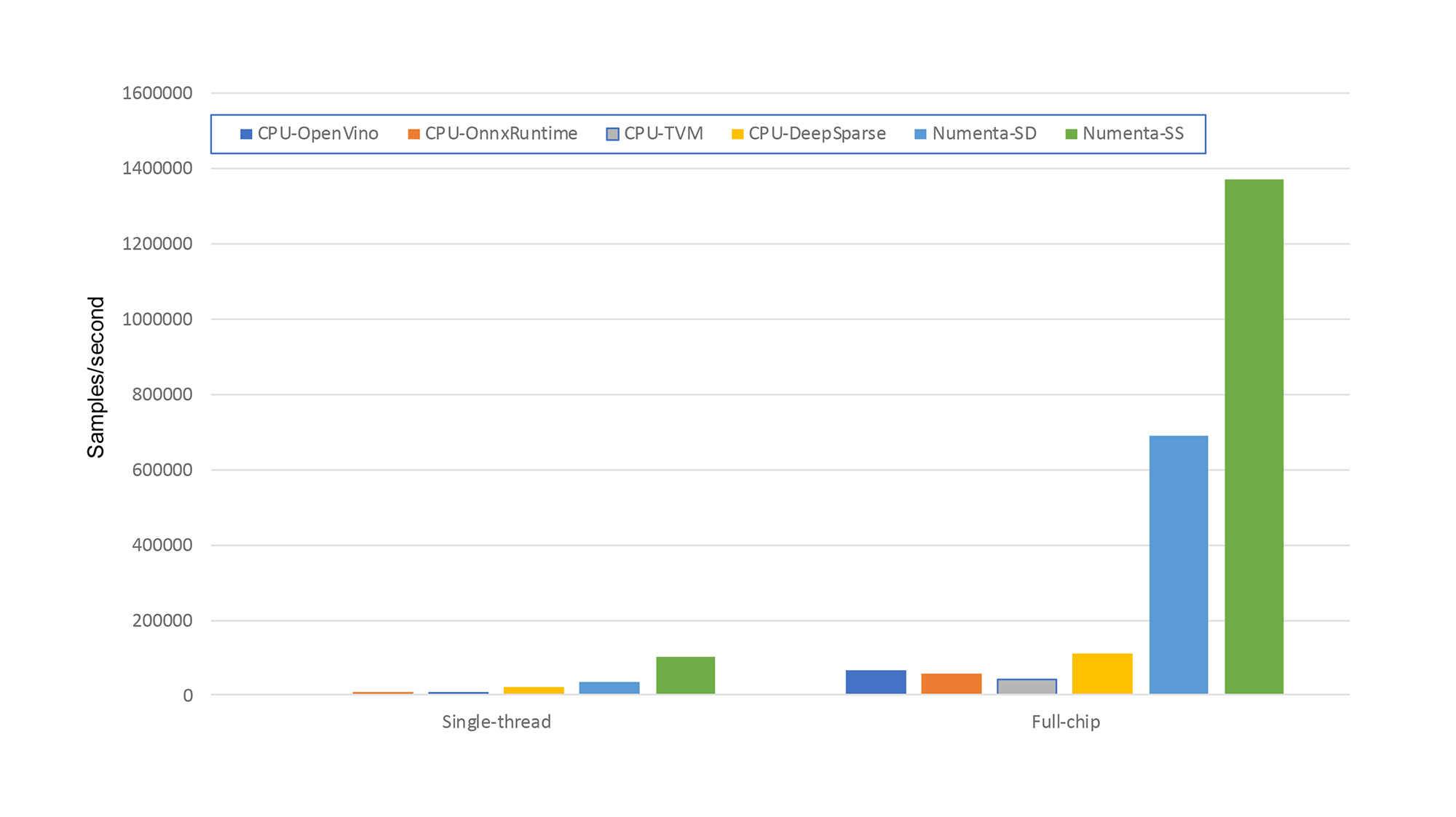
There are a variety of interesting observations from Figure 4.

• The sparse network running on the FPGA outperforms the 24-core CPU. By a lot! In fact, the FPGA sparse-sparse (Numenta-SS) network outperforms the best CPU result by over 12X. Even the slower sparse-dense network on the FPGA outperforms the CPU by 6X!
• Although it is a little hard to discern, for both the OpenVINO and OnnxRuntime there is ZERO performance improvement observed when moving to the sparse networks. This observation does not appear to be specific to this model, and it appears that these engines fail to leverage the benefits of sparsity at present!
• Both TVM and Deep Sparse leverage the sparsity of the model. For TVM, sparsity in GSC networks’ convolutional layers cannot be exploited at present, and the performance improvement is limited to the linear layers.

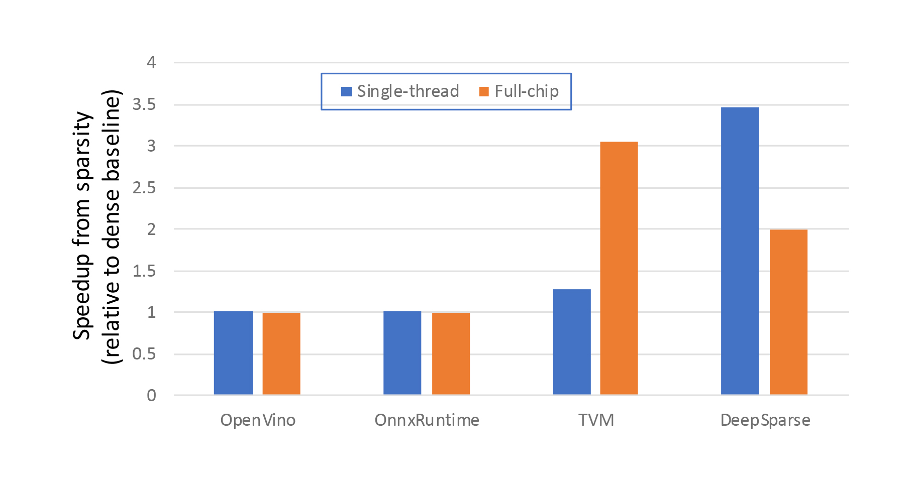
While it is encouraging that the TVM and Deep Sparse engines leverage the network sparsity to reduce inference costs, the performance benefits obtained by leveraging sparsity on CPUs are significantly more limited than observed on the FPGA, as illustrated in Figure 5. Unfortunately, the performance improvement observed for the sparse GSC network on the CPU (i.e., 2-3X) is not atypical, and the performance improvements discussed in the literature are in a similar range. This 2-3X is in stark contrast to the 112X achieved on the FPGA. The reasons for this significant discrepancy are two-fold:

• As discussed in my previous blog, the effectively random locations of the zero-valued weights and activations introduced by sparsity are difficult to exploit efficiently on CPUs with wide vector engines geared toward dense computation. For computations on 8-bit weights and activations, the vector VNNI instructions enable 64 multiply-accumulate (MAC) operations to be performed via a single instruction. Accordingly, at the sparsity levels discussed (1 in 20 elements being non-zero), even minor overheads associated with explicitly targeting and processing the non-zero overheads rapidly erode performance advantages in comparison to a brute force dense computation. This is in stark contrast to the situation on the FPGA, where its flexible nature allows sparsity to be efficiently exploited.
• The sparse-sparse network on the FPGA simultaneously leverages both weight and activation sparsity. Leveraging both dimensions of sparsity in parallel provides a multiplicative reduction in the number of computations required to perform the inference, allowing enabling extremely significant performance improvement on the FPGA.

Summary

Let’s summarize what was discussed:

• Deep neural networks are typically ‘dense’ and computationally intensive.
• It is possible to create ‘Sparse’ neural networks that match the accuracy of the dense networks but typically require between 10X to 100X fewer computations to compute a result. Ideally, we would expect to see a performance improvement and/or power saving commensurate with this reduction.
• Network weights and activations can be quantized from the typical 32-bit floating point representations to 8-bit integers. This not only reduces the memory footprint of the model but also provides acceleration on systems with vector instructions that can often process 4X more operations in parallel.
• Unfortunately, the improvements from quantization for the GSC CNN network were mixed and robust support for quantized ONNX models on CPUs still seems to be evolving.
• A comparison of dense GSC network performance on a CPU and an FPGA showed CPUs in a very favorable light. CPUs are optimized for dense, regular computations and excel at executing dense networks.
• The performance benefits observed for sparse networks on CPUs are sadly muted. For a 95% sparse CNN, which corresponds to a 20X reduction in neural weights, the improvement in inference performance was limited to around 2-3X. In fact, for two of the most well-known CPU inference engines, there was ZERO improvement relative to the dense model. This is not an aberration, and these speedups are in line with what is typically observed for sparse networks on CPUs.
• On the FPGA, Numenta achieved a 112X performance improvement from sparsity. Not only is the relative speedup from sparsity impressive, Numenta’s sparse-sparse network running on the FPGA outperformed a sparse network running on a 24-core CPU by over 12X.

In conclusion, the impressive performance benefits from sparsity achieved on the FPGA, both in relative and absolute terms, clearly demonstrate the potential for sparse models. Unfortunately, while the flexible nature of the FPGA makes it an ideal platform for sparse models, CPUs, optimized for regular, dense computations, are observed to struggle to efficiently exploit the computational reductions introduced by sparsity. New sparse techniques are needed to be able to realize more substantial performance benefits on CPUs.

In subsequent blogs, I will not only contrast the performance of sparse networks on GPUs, but also discuss how using Numenta’s sparse techniques allow controlled placement of non-zero elements in the sparse networks, while maintaining the accuracy of the model, allowing the creation of sparse models that are better suited to efficient execution on CPUs… Stay tuned…